Tutorial: Differentiable Sampling of Molecular Geometries with Uncertainty-based Adversarial Attacks
Daniel Schwalbe-Koda*
↓ SCROLL TO BEGIN ↓
Understanding material behavior
A potential energy surface (PES) describes the energy of a system based on the configuration of atoms within it. PESes are crucial in the study of materials science for understanding how materials will behave under varying conditions.
Creating accurate models of these PESes means we can discover and use better materials in many different applications--from characterizing drug activity and toxicity, to creating stronger steel compositions for spacecrafts!
Traditionally, computationally expensive methods such as ab initio simulations are used to map potential PESes. However, these methods quickly become prohibitive when a larger number of materials are screened.
Recent advances in machine learning techniques allow for high-accuracy predictions in less time and at lower costs.
Let's take a look at how this works...
Neural networks
One machine learning tool, the neural network (NN), is especially well suited to handle the extensive datasets needed to train PESes for complex materials.
NNs is typically trained on data from quantum chemistry simulations, which are considered the "ground truth" result for these predictions.
The trained neural network is then used to make predictions on that system's PES for any given geometry.
But are these predictions accurate?
Prediction error in neural networks
There is always some error associated to NN predictions. Consider the neural network on the right, which classifies whether an input image represents a dog or a cat.
Hover over the three different input photos to see what the NN predicts...
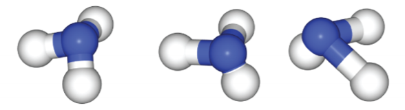
Neural networks predicting PESes face similar challenges to those outlined in the example above. While the algorithm interpolates between existing data points very well (similar to the cat and dog), it may fail catastrophically for cases for which we have little to no data (similar to the bird).
Hover over the three different input geometries to see how the network makes a prediction under uncertainty:
One problem, therefore, is: how to assess the reliability of neural network predictions?
Uncertainty Quantification
Instead of using a single neural network to make predictions, we can use an ensemble of neural networks. When the data is well-represented in the training set, the neural network committee predicts a single value with low uncertainty. On the other hand, when the data is not well-known, the NNs will disagree on the predicted property, thus leading to a higher uncertainty.
In the case of molecular simulation, it is more interesting to use uncertainty in the predicted forces instead of predicted energy.
Now, the follow-up question: how do we improve the robustness of neural networks for atomistic simulations?
Adversarial Attacks
Improving the robustness of neural network potentials requires increasing the breadth of their training sets; however, gathering this data usually requires time-consuming and costly simulations. It is therefore crucial to only gather data that will significantly improve the model's ability to make accurate predictions.
We use the concept of adversarial attacks from the machine learning literature to find which molecular geometries the NNs fail to predict. In atomistic simulations, that corresponds to adding a small disturbance δ to the input geometry and finding which are the distortions that maximize the uncertainty of the neural network committee.
Next, we exemplify how this method works...
Exemplifying adversarial attacks
Consider a 2D potential energy surface such as the one shown on the right. A toy example could be the 2D double well, which is a potential having two energy states. We can train a neural network committee to predict this potential energy surface and then analyze the energies and forces predicted by the committee.
Say that, after training the neural networks, we obtain the predictions and uncertainties on the right. The plot on the left indicates the mean energy predicted by the ensemble, while the plot on the right depicts a metric of uncertainty.
The neural networks were trained having very little information about the rightmost basin of the double well, but several data points on the left basin. As a consequence, the uncertainty is much higher on the right than on the left.
A point close to the training set is likely to have low uncertainty and a reliable PES. The NNs know this region well, and the committee agrees on which should be the predicted energy/forces.
An adversarial attack consists of distorting any predicted point to maximize the predicted uncertainty, i.e. the disagreement between the NNs. This point is likely to not be well-represented in the training set, and should be the most informative to calculate using more expensive methods.
How do we incorporate the information learned from adversarial attacks back into the original model?
Active Learning
To improve the performance of the neural network predictions, we can repeat this process in what is called an active learning loop. We start by gathering the data from a training set and training the NNs. Then, we find which are the points that maximize the committee uncertainty and send the new data for evaluation. By repeating this process, we successively improve the predictions of the NNs for the PES without human intervention.
As we execute the loop iteratively, the neural networks predict a better potential energy surface and the overall predicted uncertainty gets lower. The figure shows the evolution of the predictions, the training points points and adversarial attacks.
Change the slider below to see how the PES evolves with the number of times the loop is executed (active learning generation).